What is a Z-Score?

The z-score tells us the position of a value within data distribution using the center and spread of the distribution. Specifically, the z-score measures how many standard deviations a value is from the mean. We can use the below formula to calculate it:

• Calculating the Z-score as above is called standardization because it gives us the distance between the value and the mean in terms of standard deviations.
• A positive z-score tells us that the value is greater than the mean. In contrast, a value below the mean will produce a negative z-score.

Where:

• X = individual data point
• μ = mean of the data
• σ = standard deviation of the data

🎯 Interpretation:

• Z=0: Data point is equal to the mean.
• Z=1: 1 standard deviation above the mean.
• Z=−2: 2 standard deviations below the mean.
• Outliers are typically those with Z-scores greater than +3 or less than -3.

Let’s take an example. Suppose a newborn elephant weighed 250 pounds. You did some research and found that the average birth weight of an elephant is 200 pounds, and the standard deviation is 50 pounds.

We can use this information to calculate the z-score of the newborn elephant:

The baby elephant was born with a weight that’s exactly one standard deviation above the mean weight.

Note that the z-score of the mean value will be 0. You can verify that by plugging in the mean weight (200) in the z-score equation:

You can also do the reverse calculation to get the value for a given z-score. Simply multiply the z-score by the standard deviation and then add that to the mean. Here’s the formula:

Suppose the birth weight of another elephant had a z-score of -0.5. What’s the actual weight in pounds? Let’s find out using the above formula:

The importance of z-score becomes apparent when we use it with certain statistical distributions. Let’s look at one such example.

Z-scores and Normal Distribution

Normal distribution has some unique properties that make it well-suited for analysis using z-scores.

When we convert all values of a normally distributed variable to z-scores, we create what is known as a standard normal distribution. This new distribution will have a mean of 0 and a standard deviation of 1. Let’s look at a few properties of this distribution.

• Center at Z-score = 0

The normal distribution is centered at the mean. Since the standard normal distribution has 0 as the mean, the z-score of 0 will lie at the center.

• Symmetry

Mean splits the normal distribution into two symmetrical halves that mirror each other. Thus, the area under the curve from the center to a positive z-score, such as [0,+1.5][0,+1.5], is equal to the area between the center and the corresponding negative z-score of the same magnitude, [−1.5,0][−1.5,0].

The area under the curve represents the probability of a value falling within a specific interval. Therefore, the

two shaded z-score intervals have the same probability. In other words, if you select a random value from a normal distribution, it is equally likely to fall within the interval of [0,+1.5] as it is to fall within [−1.5,0]

Cumulative Probability and Percentile

Cumulative probability is the probability of selecting a random value that is less than or equal to a specific value.

How can we find the cumulative probability of a given z-score in a normal distribution? It’ll be equal to the proportion of area under the curve that lies to the left of the z-score. The below graph highlights this area for a z-score of 0.250.25:

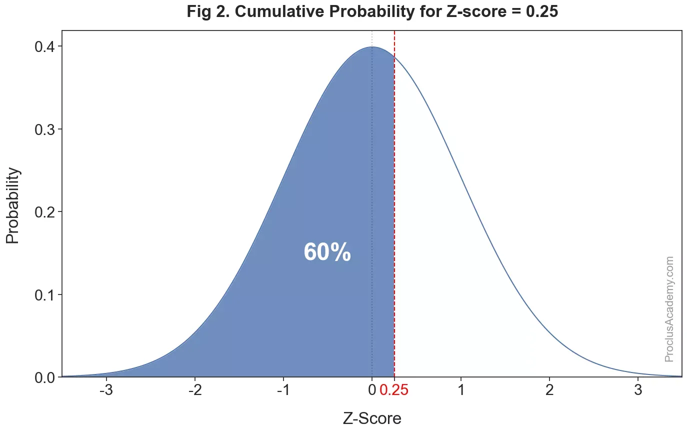
It’s roughly 60% of the total area. Hence the cumulative probability for z-score of  0.25 is about 0.60.

We can interpret this conclusion in another way - approximately 60% of the values have a z-score lower than 0.250.25. Or we could say that a z-score of 0.250.25 represents the 6060th percentilein a normal distribution.

In the example above, I estimated the shaded area to find the cumulative probability and the percentile. You can get their precise values for any given z-score by using the z-score tables or Python with the SciPy library.

Assignment: Review the empirical rule, which tells us the percentage of values that fall within 1, 2, and 3 standard deviations of the mean in a normal distribution. Can you restate this rule in terms of z-scores?

Understanding Relative Performance Using Z-score

Let’s say:

• You scored 80 in a test where the class mean was 75, and the standard deviation was 10.
• Sunny scored 65 in his class where the mean was 55, and the standard deviation was also 10.

At first glance, it might look like you performed better because 80 > 65. But in statistics, we don’t just look at raw scores — we compare how far each score is from its own class average. This is what the Z-score helps us do. Z-score can help us compare values from two different distributions.

• We need to look at how the scores are distributed in each class. Specifically, we can compare how far each score is from the mean of its respective distribution.
• Suppose both sets of scores are normally distributed. The mean and standard deviation of the scores in your class were 75 and 10, respectively. In Sunny’s class, the mean score was 55 with a standard deviation of 10.

Let’s calculate the z-score for each of your scores:

What Do These Z-scores Mean?

A Z-score tells us how many standard deviations a score is above or below the mean.

• A Z-score of 0.5 means your score is 0.5 standard deviations above your class average.
• A Z-score of 1.0 means Sunny’s score is 1 full standard deviation above his class average.

Even though your raw score is higher, Sunny’s score is farther from the mean of his class than yours is from your class.

To add even more context, statisticians use something called the cumulative probability (or percentile), which tells you the percentage of people who scored below a certain Z-score. Based on standard tables:

From a Z-table:

• A Z-score of 0.5 means you scored higher than about 69% of your classmates.
• A Z-score of 1.0 means Sunny scored higher than about 84% of his classmates.

So when you compare the two percentiles, Sunny actually outperformed more of his peers than you did, despite having a lower raw score. That’s the power of Z-scores — they level the playing field and let us compare scores from different groups fairly. In this case, Sunny might not have scored higher in absolute terms, but statistically speaking, he has a solid case for bragging rights.

This shows why context matters in statistics. Performance should always be interpreted relative to the group, not just in absolute terms.

Finding Outliers Using Z-Scores

An outlier is an extreme value that occurs far away from the bulk of the observations. Such values are either too big or too small compared to the rest of the values.

Outliers can negatively affect data analysis - they can assert undue influence on statistics such as mean and standard deviation and give you a distorted picture of how data is distributed. Hence, outlier detection is one of the most crucial steps in data analysis.

The question is - how can we detect outliers? As per the empirical rule, 99.7% of the values of a normal distribution fall within 3 standard deviations from the mean. Any value outside of this range is considered an outlier because the probability of getting such a value is only 0.3% - a rarity.

Let me explain this using an example. Suppose you collect data on 200 basketball players for a season and calculate the average number of points they scored per game. And then plot average points per game as a histogram:

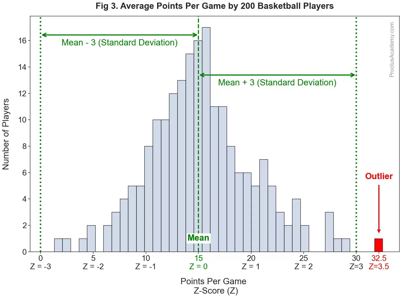
• The average points per game are almost normally distributed - a slight variation from the theoretical, smooth curve is expected with real world data. The distribution has a mean of 15 with a standard deviation of 5. Thus, the points per game for most players are in the vicinity of 15.
• We can also convert the points per game to z-score. Thus, the mean (15) will have a z-score of 0, and 20 will translate to a z-score of 1, etc. The graph shows the z-scores below the raw points per game on the x-axis.
• Almost all the values fall within 3 standard deviations, or within the z-score range of [−3.0,+3.0].
• However, one player finished the season with 32.5 points per game, which translates to a z-score of 3.53. His score is far from the rest of the players and lies beyond the range of 3 standard deviations from the mean. We’ll get such performance very rarely and thus consider it an outlier.

Once we’ve found outliers, we can handle them in many different ways. We can either exclude them from analysis or use measures such as the median, which are not unduly affected by the outliers. See my related post on this topic.

Summary

This article introduced you to the concept of z-score using practical, real-life examples. Let’s quickly recap what you learned today:

• What is z-score, and how does it help us understand the relative position of an observation within a distribution.
• What are the special properties of normal distribution (symmetry, predictable area under the curve), and how can we use z-scores and these properties to calculate probabilities and percentiles.
• How can we use z-scores to compare values from different yet similar distributions?
• What are outliers, and why is it important to identify them. How can z-score help usdetect outliers in normally distributed data.

2. Z-Score Outlier Detection: Single Column

This method is ideal when analyzing a specific numeric feature, such as "sales", "revenue", or "price".

Step-by-Step Process:

import numpy as np
import pandas as pd
from scipy import stats


# Detect Z-score outliers for a single column
def detect_outliers_zscore(data, threshold=3):
    z_scores = np.abs(stats.zscore(data))
    outlier_mask = z_scores > threshold
    
    return outlier_mask, z_scores

Example:

# Assume 'df' is your DataFrame and 'value' is the column of interest
outlier_mask, z_scores = detect_outliers_zscore(df['value'], threshold=3)

# View outliers
outliers_df = df[outlier_mask].copy()
outliers_df['z_score'] = z_scores[outlier_mask]

# Remove outliers
df_clean = df[~outlier_mask].copy()

print(f"Outliers detected: {outlier_mask.sum()} ({(outlier_mask.sum()/len(df))*100:.2f}%)")
print(f"Clean dataset shape: {df_clean.shape}")

3. Z-Score Outlier Detection: Multiple Columns

In practice, datasets often contain many numeric variables. Here, the method applies Z-score logic to each numeric column individually.

🔁 Process Summary:

1. Loop through all numeric columns.
2. Compute Z-scores.
3. Flag values as outliers if Z > threshold.
4. Optionally remove rows with outliers or store results for analysis.

✅ Implementation:

python
CopyEdit
outlier_dfs = []
df_clean = df.copy()

for col in df.select_dtypes(include=[np.number]).columns:
    outlier_mask, z_scores = detect_outliers_zscore(df[col])

    outliers_df = df[outlier_mask].copy()
    outliers_df['column'] = col
    outliers_df['z_score'] = z_scores[outlier_mask]
    outliers_df['value'] = df[col][outlier_mask]
    outlier_dfs.append(outliers_df)

    df_clean = df_clean[~outlier_mask]

# Combine all outliers
all_outliers_df = pd.concat(outlier_dfs).sort_values(['column', 'z_score'], ascending=[True, False])

# Output
print(f"Total outliers found: {len(all_outliers_df)}")
print(f"Cleaned dataset shape: {df_clean.shape}")

📘 Summary Table

💡 Best Practices for Practitioners

• Use Z-score method only on normally distributed features. For skewed data, consider IQR, Isolation Forest, or Robust Scaler.
• Always visualize data distribution before applying outlier detection.
• For time-series data, Z-scores may mislead due to non-stationarity.
• Never blindly drop outliers — assess their business context (e.g., a very high revenue may be legitimate).
• For high-dimensional datasets, consider Mahalanobis distance or multivariate methods.

📎 Example Use Case in Finance

If you're analyzing monthly expenses, an unusually large transaction with a Z-score of +4 could indicate fraud, a rare investment, or a posting error.

Question to Ask:

Is this outlier informative or an error?

Do I flag it, remove it, or keep it for risk analysis?

Z-Score Outlier Detection: Complete Guide with Real Dataset

What is Z-Score Outlier Detection?

Z-Score outlier detection identifies data points that are unusually far from the mean of a dataset. It measures how many standard deviations a data point is from the mean. The formula is:

Z = (X - μ) / σ

Where:

• X = individual data point
• μ = mean of the dataset
• σ = standard deviation of the dataset

Common thresholds:

• |Z| > 2: Moderate outlier (≈95% of data falls within 2 standard deviations)
• |Z| > 3: Strong outlier (≈99.7% of data falls within 3 standard deviations)

Why Use Z-Score Detection?

Advantages:

• Simple and interpretable
• Works well with normally distributed data
• Computationally efficient
• Provides a standardized measure across different scales

Limitations:

• Assumes normal distribution
• Sensitive to extreme outliers (can mask other outliers)
• May not work well with skewed data
• Treats all features equally regardless of their importance

Implementation: Single Column Analysis

Let’s start with a practical example using the California Housing dataset:

import numpy as np
import pandas as pd
from scipy import stats
import matplotlib.pyplot as plt
import seaborn as sns
from sklearn.datasets import fetch_california_housing
import warnings
warnings.filterwarnings('ignore')

# Load the dataset
housing = fetch_california_housing()
df = pd.DataFrame(housing.data, columns=housing.feature_names)
df['target'] = housing.target

print("Dataset shape:", df.shape)
print("\\nFirst few rows:")
print(df.head())
print("\\nDataset info:")
print(df.describe())

Step 1: Create Z-Score Detection Function

def detect_outliers_zscore(data, threshold=3):
    """
    Detect outliers using Z-score method

    Parameters:
    data: pandas Series or numpy array
    threshold: Z-score threshold (default=3)

    Returns:
    outlier_mask: Boolean mask where True indicates outlier
    z_scores: Z-scores for all data points
    """
    # Calculate Z-scores
    z_scores = np.abs(stats.zscore(data))

    # Create outlier mask
    outlier_mask = z_scores > threshold

    return outlier_mask, z_scores

Step 2: Analyze Single Column (House Values)

# Analyze house values (target variable)
column_name = 'target'
outlier_mask, z_scores = detect_outliers_zscore(df[column_name], threshold=3)

# Create results DataFrame
outliers_df = df[outlier_mask].copy()
outliers_df['z_score'] = z_scores[outlier_mask]

# Display results
print(f"Analysis for column: {column_name}")
print(f"Total data points: {len(df)}")
print(f"Outliers detected: {outlier_mask.sum()} ({(outlier_mask.sum()/len(df))*100:.2f}%)")
print(f"Outlier threshold: |Z| > 3")

print("\\nTop 10 outliers:")
print(outliers_df.nlargest(10, 'z_score')[['target', 'z_score']])

# Visualize the distribution
plt.figure(figsize=(15, 5))

# Original distribution
plt.subplot(1, 3, 1)
plt.hist(df[column_name], bins=50, alpha=0.7, color='skyblue', edgecolor='black')
plt.axvline(df[column_name].mean(), color='red', linestyle='--', label=f'Mean: {df[column_name].mean():.2f}')
plt.title(f'Original Distribution: {column_name}')
plt.xlabel('House Value (100k USD)')
plt.ylabel('Frequency')
plt.legend()

# Z-scores distribution
plt.subplot(1, 3, 2)
plt.hist(z_scores, bins=50, alpha=0.7, color='lightgreen', edgecolor='black')
plt.axvline(3, color='red', linestyle='--', label='Threshold: Z=3')
plt.axvline(-3, color='red', linestyle='--')
plt.title('Z-Scores Distribution')
plt.xlabel('Z-Score')
plt.ylabel('Frequency')
plt.legend()

# Box plot showing outliers
plt.subplot(1, 3, 3)
box_plot = plt.boxplot(df[column_name], patch_artist=True)
box_plot['boxes'][0].set_facecolor('lightcoral')
plt.title(f'Box Plot: {column_name}')
plt.ylabel('House Value (100k USD)')

plt.tight_layout()
plt.show()

# Remove outliers and compare
df_clean_single = df[~outlier_mask].copy()
print(f"\\nAfter removing outliers:")
print(f"Clean dataset shape: {df_clean_single.shape}")
print(f"Original mean: {df[column_name].mean():.2f}")
print(f"Clean mean: {df_clean_single[column_name].mean():.2f}")
print(f"Original std: {df[column_name].std():.2f}")
print(f"Clean std: {df_clean_single[column_name].std():.2f}")

Implementation: Multiple Columns Analysis

Now let’s extend this to analyze all numeric columns simultaneously:

def detect_outliers_multiple_columns(df, threshold=3, exclude_columns=None):
    """
    Detect outliers across multiple numeric columns

    Parameters:
    df: pandas DataFrame
    threshold: Z-score threshold
    exclude_columns: list of columns to exclude from analysis

    Returns:
    outlier_summary: DataFrame with outlier statistics per column
    all_outliers_df: Combined DataFrame of all outliers
    df_clean: DataFrame with outliers removed
    """
    if exclude_columns is None:
        exclude_columns = []

    # Get numeric columns
    numeric_cols = df.select_dtypes(include=[np.number]).columns
    numeric_cols = [col for col in numeric_cols if col not in exclude_columns]

    outlier_dfs = []
    outlier_summary = []
    df_clean = df.copy()

    for col in numeric_cols:
        # Detect outliers for this column
        outlier_mask, z_scores = detect_outliers_zscore(df[col], threshold)

        # Store outlier information
        if outlier_mask.sum() > 0:
            outliers_df = df[outlier_mask].copy()
            outliers_df['column'] = col
            outliers_df['z_score'] = z_scores[outlier_mask]
            outliers_df['outlier_value'] = df[col][outlier_mask]
            outlier_dfs.append(outliers_df[['column', 'z_score', 'outlier_value']])

        # Store summary statistics
        outlier_summary.append({
            'column': col,
            'total_outliers': outlier_mask.sum(),
            'outlier_percentage': (outlier_mask.sum() / len(df)) * 100,
            'max_z_score': z_scores.max(),
            'min_value': df[col].min(),
            'max_value': df[col].max(),
            'mean_value': df[col].mean(),
            'std_value': df[col].std()
        })

        # Remove outliers from clean dataset
        df_clean = df_clean[~outlier_mask]

    # Combine all outliers
    all_outliers_df = pd.concat(outlier_dfs) if outlier_dfs else pd.DataFrame()
    if not all_outliers_df.empty:
        all_outliers_df = all_outliers_df.sort_values(['column', 'z_score'], ascending=[True, False])

    # Create summary DataFrame
    outlier_summary_df = pd.DataFrame(outlier_summary)

    return outlier_summary_df, all_outliers_df, df_clean

# Apply to our dataset
outlier_summary, all_outliers, df_clean_multiple = detect_outliers_multiple_columns(df, threshold=3)

print("=== OUTLIER SUMMARY BY COLUMN ===")
print(outlier_summary.round(2))

print(f"\\n=== OVERALL RESULTS ===")
print(f"Original dataset shape: {df.shape}")
print(f"Clean dataset shape: {df_clean_multiple.shape}")
print(f"Total outliers found: {len(all_outliers)}")
print(f"Rows removed: {len(df) - len(df_clean_multiple)}")

# Display top outliers by column
print(f"\\n=== TOP 5 OUTLIERS BY COLUMN ===")
for col in outlier_summary['column'].head():
    col_outliers = all_outliers[all_outliers['column'] == col].head()
    if not col_outliers.empty:
        print(f"\\n{col}:")
        print(col_outliers[['z_score', 'outlier_value']].round(2))

Visualization: Before and After Comparison

# Create comprehensive visualization
def visualize_outlier_detection(df_original, df_clean, columns_to_plot=None):
    """
    Visualize the effect of outlier removal
    """
    if columns_to_plot is None:
        columns_to_plot = df_original.select_dtypes(include=[np.number]).columns[:4]

    fig, axes = plt.subplots(2, len(columns_to_plot), figsize=(20, 10))

    for i, col in enumerate(columns_to_plot):
        # Before outlier removal
        axes[0, i].hist(df_original[col], bins=30, alpha=0.7, color='lightcoral', edgecolor='black')
        axes[0, i].set_title(f'Before: {col}')
        axes[0, i].set_xlabel(col)
        axes[0, i].set_ylabel('Frequency')

        # After outlier removal
        axes[1, i].hist(df_clean[col], bins=30, alpha=0.7, color='lightgreen', edgecolor='black')
        axes[1, i].set_title(f'After: {col}')
        axes[1, i].set_xlabel(col)
        axes[1, i].set_ylabel('Frequency')

    plt.tight_layout()
    plt.show()

# Visualize key columns
key_columns = ['MedInc', 'HouseAge', 'AveRooms', 'target']
visualize_outlier_detection(df, df_clean_multiple, key_columns)

Advanced: Handling Different Data Types

def smart_outlier_detection(df, threshold=3, auto_transform=True):
    """
    Smart outlier detection with automatic handling of skewed data
    """
    results = {}
    numeric_cols = df.select_dtypes(include=[np.number]).columns

    for col in numeric_cols:
        # Check if data is normally distributed
        _, p_value = stats.normaltest(df[col])
        is_normal = p_value > 0.05

        if is_normal or not auto_transform:
            # Use standard Z-score
            outlier_mask, z_scores = detect_outliers_zscore(df[col], threshold)
            method = 'Standard Z-score'
        else:
            # Use log transformation for skewed data
            try:
                log_data = np.log1p(df[col] - df[col].min() + 1)
                outlier_mask, z_scores = detect_outliers_zscore(log_data, threshold)
                method = 'Log-transformed Z-score'
            except:
                # Fallback to standard method
                outlier_mask, z_scores = detect_outliers_zscore(df[col], threshold)
                method = 'Standard Z-score (fallback)'

        results[col] = {
            'outlier_mask': outlier_mask,
            'z_scores': z_scores,
            'method': method,
            'is_normal': is_normal,
            'outlier_count': outlier_mask.sum(),
            'outlier_percentage': (outlier_mask.sum() / len(df)) * 100
        }

    return results

# Apply smart detection
smart_results = smart_outlier_detection(df, threshold=3)

print("=== SMART OUTLIER DETECTION RESULTS ===")
for col, result in smart_results.items():
    print(f"\\n{col}:")
    print(f"  Method: {result['method']}")
    print(f"  Normal distribution: {result['is_normal']}")
    print(f"  Outliers: {result['outlier_count']} ({result['outlier_percentage']:.2f}%)")

Best Practices and Recommendations

1. When to Use Z-Score Detection

• Good for: Normally distributed data, quick screening, standardized comparison
• Avoid for: Highly skewed data, small datasets (<30 samples), categorical data

2. Choosing the Right Threshold

# Different threshold analysis
thresholds = [2, 2.5, 3, 3.5]
threshold_results = {}

for threshold in thresholds:
    outlier_mask, _ = detect_outliers_zscore(df['target'], threshold)
    threshold_results[threshold] = {
        'outlier_count': outlier_mask.sum(),
        'outlier_percentage': (outlier_mask.sum() / len(df)) * 100
    }

threshold_df = pd.DataFrame(threshold_results).T
print("Threshold Impact Analysis:")
print(threshold_df.round(2))

3. Business Context Considerations

def business_context_analysis(df, outliers_df, column_name):
    """
    Analyze outliers in business context
    """
    print(f"=== BUSINESS CONTEXT ANALYSIS: {column_name} ===")

    # Statistical summary
    print(f"Normal range (within 2 std): {df[column_name].mean() - 2*df[column_name].std():.2f} to {df[column_name].mean() + 2*df[column_name].std():.2f}")

    # Outlier characteristics
    high_outliers = outliers_df[outliers_df[column_name] > df[column_name].mean()]
    low_outliers = outliers_df[outliers_df[column_name] < df[column_name].mean()]

    print(f"High-value outliers: {len(high_outliers)}")
    print(f"Low-value outliers: {len(low_outliers)}")

    # Recommendations
    print("\\nRecommendations:")
    if column_name == 'target':
        print("- High-value outliers might be luxury properties or data errors")
        print("- Low-value outliers could indicate distressed sales or unique locations")
        print("- Consider keeping outliers for model training to capture full market range")

    return high_outliers, low_outliers

# Apply business context analysis
target_outliers = df[detect_outliers_zscore(df['target'], threshold=3)[0]]
high_outliers, low_outliers = business_context_analysis(df, target_outliers, 'target')

Summary and Decision Framework

Quick Decision Tree:

1. Is your data normally distributed? → Use Z-score
2. Is your data skewed? → Consider log transformation or IQR method
3. Do you have domain knowledge? → Set custom thresholds
4. Are outliers meaningful? → Keep them for analysis
5. Are outliers errors? → Remove them carefully

Final Recommendations:

• Always visualize your data before and after outlier removal
• Consider multiple detection methods and compare results
• Document your outlier handling decisions
• Test your model performance with and without outliers
• Remember: Not all outliers are bad - some contain valuable information!

# Final comparison summary
print("=== FINAL COMPARISON SUMMARY ===")
print(f"Original dataset: {df.shape}")
print(f"After single-column cleaning: {df_clean_single.shape}")
print(f"After multi-column cleaning: {df_clean_multiple.shape}")
print(f"Percentage of data retained: {(len(df_clean_multiple)/len(df))*100:.1f}%")

This comprehensive approach ensures you understand both the technical implementation and business implications of Z-score outlier detection.

Assumption of Z-score

The z-score method for outlier detection, while widely used due to its simplicity, has several significant limitations that stem from its underlying assumptions and mathematical properties. Core Assumptions The z-score method assumes that data follows a normal distribution. This is perhaps the most critical assumption, as z-scores are calculated based on the mean and standard deviation, which are optimal measures of central tendency and spread only for normally distributed data. When data is skewed, multimodal, or follows other distributions, z-scores become unreliable indicators of outliers. The method also assumes that outliers are points that fall beyond a certain number of standard deviations from the mean (typically 2 or 3). This threshold is derived from the properties of the normal distribution, where approximately 95% of data falls within 2 standard deviations and 99.7% within 3 standard deviations. Major Limitations Sensitivity to the outliers themselves represents a fundamental flaw in the z-score approach. Since both the mean and standard deviation are calculated using all data points, extreme outliers can significantly influence these statistics. This creates a masking effect where the presence of outliers inflates the standard deviation and shifts the mean, making other outliers appear less extreme and potentially missing them entirely. Inability to handle skewed distributions is another critical limitation. In right-skewed data, for example, the mean is pulled toward the tail, and the standard deviation is inflated. This can cause legitimate high values to be incorrectly flagged as outliers, while true outliers in the shorter tail might be missed. Poor performance with small sample sizes occurs because the sample mean and standard deviation become unreliable estimates of population parameters when n is small. The z-score thresholds derived from normal distribution properties lose their validity, leading to either too many false positives or missed outliers. Univariate limitation means that z-scores can only detect outliers in individual variables. They cannot identify multivariate outliers - points that may appear normal in each dimension individually but are outliers when considering the correlation structure between variables. Fixed threshold rigidity is problematic because the conventional thresholds (±2 or ±3) may not be appropriate for all datasets or contexts. Different domains may require different sensitivity levels, and the optimal threshold depends on the specific distribution and the consequences of false positives versus false negatives. Distribution-Specific Issues For heavy-tailed distributions like those following a t-distribution or Cauchy distribution, the z-score method will generate excessive false positives because these distributions naturally have more extreme values than the normal distribution. Conversely, for light-tailed distributions, the method might be too conservative. In the presence of multiple outlier clusters, the z-score method struggles because it assumes a single central tendency. If outliers exist in groups, the method might miss entire clusters or incorrectly identify normal variation as outliers. Alternative Approaches Given these limitations, more robust methods are often preferable. The Interquartile Range (IQR) method is less sensitive to outliers since it uses quartiles rather than mean and standard deviation. Modified z-scores using the median absolute deviation (MAD) provide greater robustness. For multivariate data, methods like Mahalanobis distance or isolation forests are more appropriate. The z-score method works best when data is approximately normal, sample sizes are adequate, and the goal is to identify extreme values in a univariate context. However, practitioners should always examine data distribution and consider the specific context before relying solely on z-scores for outlier detection.