INTRODUCTION

The XLOOKUP function in Excel searches a range or an array for a specified value and returns the related value from another column. It can look up both vertically and horizontally and perform an exact match (default), approximate (closest) match, or wildcard (partial) match.

The syntax of the XLOOKUP function is as follows:

XLOOKUP(lookup_value, lookup_array, return_array, [if_not_found], [match_mode], [search_mode])

The first 3 arguments are required and the last three are optional.

• Lookup_value - the value to search for.
• Lookup_array - the range or array where to search.
• Return_array - the range or array from which to return values.
• If_not_found [optional] - the value to return if no match is found. If omitted, an #N/A error is returned.
• Match_mode [optional] - the match type to perform:
• 0 or omitted (default) - exact match. If not found, an #N/A error is returned.
• 1 - exact match or next smaller. If an exact match is not found, the next smaller value is returned.
• 1 - exact match or next larger. If an exact match is not found, the next larger value is returned.
• 2 - wildcard character match.
• Search_mode [optional] - the direction of search:
• 1 or omitted (default) - to search from first to last.
• 1 - to search in reverse order, from last to first.
• 2 - binary search on data sorted ascending.
• 2 - binary search on data sorted descending.

According to Microsoft, binary search is included for advanced users. It is a special algorithm that finds the position of a lookup value within a sorted array by comparing it to the middle element of the array. A binary search is much faster than a regular search but works correctly only on sorted data.

How to use XLOOKUP in Excel

The following examples demonstrate the most useful XLOOKUP features in action. Additionally, you will discover a couple non-trivial uses that will take your Excel lookup skills to a new level.

XLOOKUP with multiple criteria

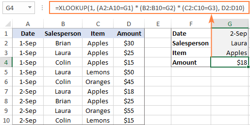
Another big advantage of XLOOKUP is that it handles arrays natively. Due to this ability, you can evaluate multiple criteria directly in the lookup_array argument:

XLOOKUP(1, (criteria_range1=criteria1) * (criteria_range2=criteria2) * (…), return_array)

How this formula works: The result of each criteria test is an array of TRUE and FALSE values. The multiplication of the arrays converts TRUE and FALSE into 1 and 0, respectively, and produces the final lookup array. As you know, multiplying by 0 always gives zero, so in the lookup array, only the items that meet all the criteria are represented by 1. And because our lookup value is "1", Excel takes the first "1" in lookup_array (first match) and returns the value from return_array in the same position.

To see the formula in action, let's pull an amount from D2:D10 (return_array) with the following conditions:

• Criteria1 (date) = G1
• Criteria2 (salesperson) = G2
• Criteria3 (item) = G3

With dates in A2:A10 (criteria_range1), salesperson names in B2:B10 (criteria_range2) and items in C2:C10 (criteria_range3), the formula takes this shape:

=XLOOKUP(1, (B2:B10=G1) * (A2:A10=G2) * (C2:C10=G3), D2:D10)

Though the Excel XLOOKUP function processes arrays, it works as a regular formula and is completed with a usual Enter keystroke.

The XLOOKUP formula with multiple criteria is not limited to "equal to" conditions. You are free to use other logical operators as well. For example, to filter orders made on the date in G1 or earlier, put "<=G1" in the first criterion:

=XLOOKUP(1, (A2:A10<=G1) * (B2:B10=G2) * (C2:C10=G3), D2:D10)

For more examples, please see How to use XLOOKUP multiple criteria.

Double / nested XLOOKUP

To find a value at the intersection of a certain row and column, perform the so-called double lookup or matrix lookup. Yep, Excel XLOOKUP can do that too! You simply nest one function inside another:

XLOOKUP(lookup_value1, lookup_array1, XLOOKUP(lookup_value2, lookup_array2, data_values))

How this formula works: The formula is based on XLOOKUP's ability to return an entire row or column. The inner function searches for its lookup value and returns a column or row of related data. That array goes to the outer function as the return_array.

For this example, we are going to find the sales made by a particular salesperson within a certain quarter. For this, we enter the lookup values in H1 (salesperson name) and H2 (quarter), and do a two-way Xlookup with the following formula:

=XLOOKUP(H1, A2:A6, XLOOKUP(H2, B1:E1, B2:E6))

Or the other way round:

=XLOOKUP(H2, B1:E1, XLOOKUP(H1, A2:A6, B2:E6))

Where A2:A6 are the salesperson names, B1:E1 are quarters (column headers), and B2:E6 are data values.

A two-way lookup can also be performed with an INDEX Match formula and in a few other ways. For more information, please see Two-way lookup in Excel.

If Error XLOOKUP

When the lookup value is not found, Excel XLOOKUP returns an #N/A error. Quite familiar and understandable to expert users, it might be rather confusing for novices. To replace the standard error notation with a user-friendly message, type your own text into the 4th argument named if_not_found.

Back to the very first example discussed in this tutorial. If someone inputs an invalid ocean name in E1, the following formula will explicitly tell them that "No match is found":

=XLOOKUP(E1, A2:A6, B2:B6, "No match is found")

Notes:

• The if_not_found argument traps only #N/A errors, not all errors.
• #N/A errors can also be handled with IFNA and VLOOKUP, but the syntax is a bit more complex and a formula is lengthier.

Case-sensitive XLOOKUP

By default, the XLOOKUP function treats lowercase and uppercase letters as the same characters. To make it case-sensitive, use the EXACT function for the lookup_array argument:

XLOOKUP(TRUE, EXACT(lookup_value, lookup_array), return_array)

How this formula works: The EXACT function compares the lookup value against each value in lookup array and returns TRUE if they are exactly the same including the letter case, FALSE otherwise. This array of logical values goes to the lookup_array argument of XLOOKUP. As the result, XLOOKUP searches for the TRUE value in the above array and returns a match from the return array.

For example, to get the price from B2:B7 (return_array) for the item in E1 (lookup_value), the formula in E2 is:

=XLOOKUP(TRUE, EXACT(E1, A2:A7), B2:B7, "Not found")

Note. If there are two or more exactly the same values in the lookup array (including the letter case), the first found match is returned.

Excel XLOOKUP not working

If your formula does not work right or results in error, most likely it's because of the following reasons:

XLOOKUP is not available in my Excel

The XLOOKUP function is not backward compatible. It's only available in Excel for Microsoft 365 and Excel 2021, and won't appear in earlier versions.

XLOOKUP returns wrong result

If your obviously correct Xlookup formula returns a wrong value, chances are that the lookup or return range "shifted" when the formula was copied down or across. To prevent this from happening, be sure to always lock both ranges with absolute cell references (like $A$2:$A$10).

XLOOKUP returns #N/A error

An #N/A error just means the lookup value is not found. To fix this, try searching for approximate match or inform your users that no match is found.

XLOOKUP returns #VALUE error

A #VALUE! error occurs if the lookup and return arrays have incompatible dimensions. For instance, it is not possible to search in a horizontal array and return values from a vertical array.

XLOOKUP returns #REF error

A #REF! error is thrown when looking up between two different workbooks, one of which is closed. To fix the error, simply open both files.

As you have just seen, XLOOKUP has many awesome features that make it THE function for almost any lookup in Excel. I thank you for reading and hope to see you on our blog next week!